Case10. 顧客価値を予測する

実際にランダムフォレストを使って、顧客価値予測モデルを作成していきます。

フロー

• データセットの作成
• モデル作成用、検証用にデータセットを分離
• モデル作成用のデータセットでモデリング
• モデルでの予測値（検証用データの各要因をモデルに適用した結果）と検証用データの比較
• モデル内容

参考：
https://www.kaggle.com/snmateen/h2o-random-forest

# ライブラリの読み込み
library(data.table)
library(dplyr)
library(ggplot2)
library(stringr)
library(randomForest)

# データの読み込み
train  <- fread("./data/case10_act_train.csv", showProgress = FALSE, data.table = FALSE)
people <- fread("./data/case10_people.csv", showProgress = FALSE, data.table = FALSE)

### 前処理
# char_2と同じなので除外
people$char_1 <- NULL

# date in year, month and day
people$year  <- as.integer(substr(people$date, 1, 4))
people$month <- as.integer(substr(people$date, 6, 7))
people$day   <- as.integer(substr(people$date, 9, 10))
people <- select(people, -date)

train$year  <- as.integer(substr(train$date, 1, 4))
train$month <- as.integer(substr(train$date, 6, 7))
train$day   <- as.integer(substr(train$date, 9, 10))
train <- select(train, -date)

# 論理型をダミー変数に変換
p_logi <- names(people)[which(sapply(people, is.logical))]
for (col in p_logi) set(people, j = col, value = as.numeric(people[[col]]))

# trainとpeopleに同じカラム名があるのでカラム名を変更
names(people)[2:ncol(people)] <- paste0('people_', names(people)[2:ncol(people)])

## テーブルの結合
data <- merge(train, people, by = "people_id", all.x = T)

# IDは除外
data <- select(data, -people_id)

# カテゴリデータをダミー変数に置き換え
feature.names <- names(select(data, -outcome))
for (f in feature.names) {
  if (class(data[[f]])=="character") {
    levels <- unique(c(data[[f]]))
    data[[f]] <- as.integer(factor(data[[f]], levels=levels))
  }
}

# 0と1しかないのでファクター型に変換
data$outcome <- as.factor(data$outcome)

# すべてのデータを使うと時間がかかるので調整
model.dat <- data[1:100000,]  

# トレーニング用にサンプルをランダムに抽出
train.index <- sort(sample(1:nrow(model.dat), size = 70000))

# モデリング用と検証用にデータセットを分離
train <- model.dat[train.index,]
test  <- model.dat[-train.index,]

# この処理は時間がかかります
# チューニング
train.tune <- tuneRF(train[,feature.names], train$outcome,  doBest = T)

## mtry = 7  OOB error = 0.81%
## Searching left ...
## mtry = 4     OOB error = 1.18%
## -0.4603175 0.05
## Searching right ...
## mtry = 14    OOB error = 0.61%
## 0.2486772 0.05
## mtry = 28    OOB error = 0.53%
## 0.1220657 0.05
## mtry = 56    OOB error = 0.57%
## -0.05882353 0.05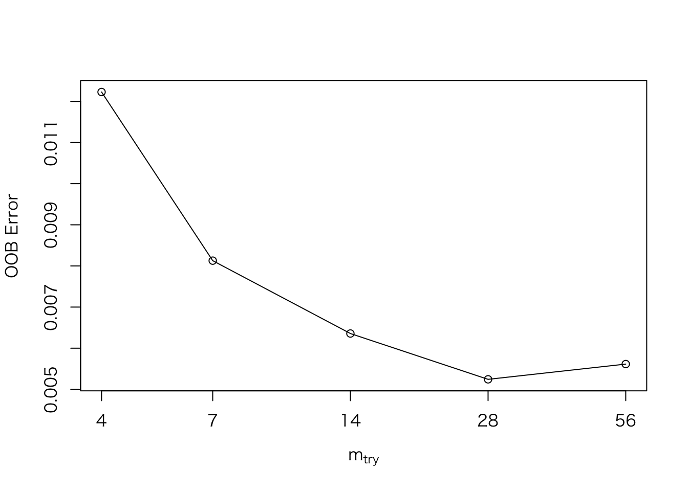

# モデリング
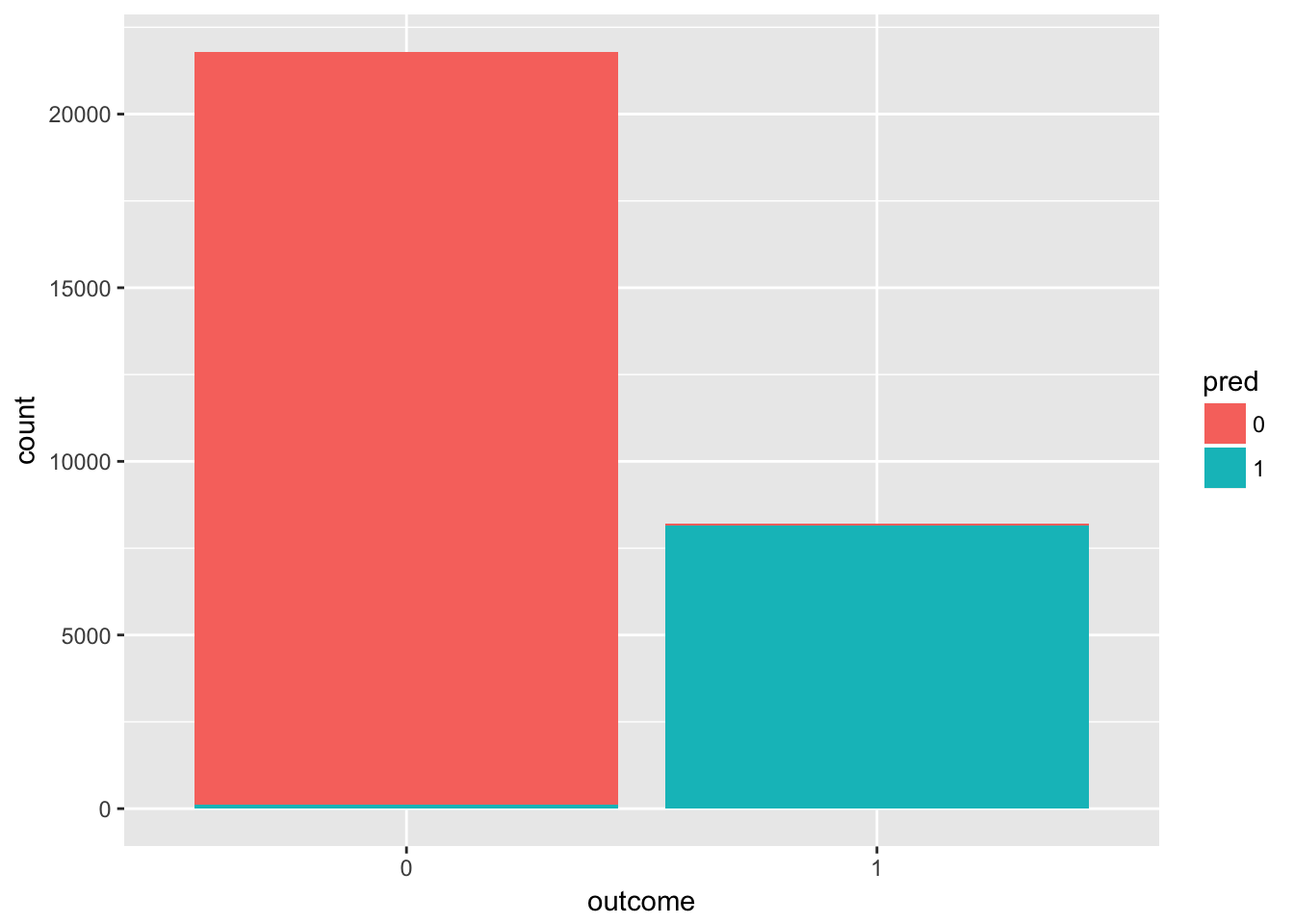
train.rf <- randomForest(outcome ~., data = train, mtry = train.tune$mtry )

# 検証用データにモデルを適用
test$pred <- predict(train.rf, test)

group_by(test,pred,outcome) %>%
  summarise(count = n()) %>%
    ggplot(aes(x = outcome, y = count, fill = pred)) +
      geom_bar(stat = "identity") 

varImpPlot(train.rf)