Case1. 売上を予測する

実際にランダムフォレストを使って、売上予測モデルを作成していきます。

フロー

データセットの作成
モデル作成用、検証用にデータセットを分離
モデル作成用のデータセットでモデリング
モデルでの予測値（検証用データの各要因をモデルに適用した結果）と検証用データの比較
モデル内容

# ライブラリの読み込み
library(data.table)
library(dplyr)
library(ggplot2)
library(randomForest)

# データの読み込み
train <- fread("./data/case01_train.csv", showProgress = FALSE, data.table = FALSE)
store <- fread("./data/case01_store.csv", showProgress = FALSE, data.table = FALSE)
train <- left_join(train, store, by = "Store")

データセットの作成

# 営業日のデータのみ使う
train <- filter(train, Open == 1)

# 欠損値は0で補完
train[is.na(train)]   <- 0

# 時系列情報を分解
train$Date <- as.Date(train$Date)
train$month <- as.integer(format(train$Date, "%m"))
train$year <- as.integer(format(train$Date, "%y"))
train$day <- as.integer(format(train$Date, "%d"))

# date, Customers, Open, StateHolidayは除外
model.dat <- select(train, -c(3, 5, 6, 8))

for (f in names(model.dat)) {
  if (class(train[[f]])=="character") {
    levels <- unique(model.dat[[f]])
    model.dat[[f]] <- as.integer(factor(model.dat[[f]], levels=levels))
  }
}

データセットの分離

# すべてのデータを使うと時間がかかるので調整
model.dat <- model.dat[1:100000,]

# トレーニング用に70000サンプルをランダムに抽出
train.index <- sort(sample(1:nrow(model.dat), size = 70000))

#モデリング用と検証用にデータセットを分離
train <- model.dat[train.index,]
test  <- model.dat[-train.index,]

モデリング

ランダムフォレストでモデリング

# この処理は時間がかかります
# チューニング
feature.names <- names(select(train, -Sales))
train.tune <- tuneRF(train[,feature.names], train$Sales,  doBest = T)

## mtry = 5  OOB error = 1474034
## Searching left ...
## mtry = 3     OOB error = 3072661
## -1.084525 0.05
## Searching right ...
## mtry = 10    OOB error = 1078813
## 0.2681224 0.05
## mtry = 16    OOB error = 1057374
## 0.01987207 0.05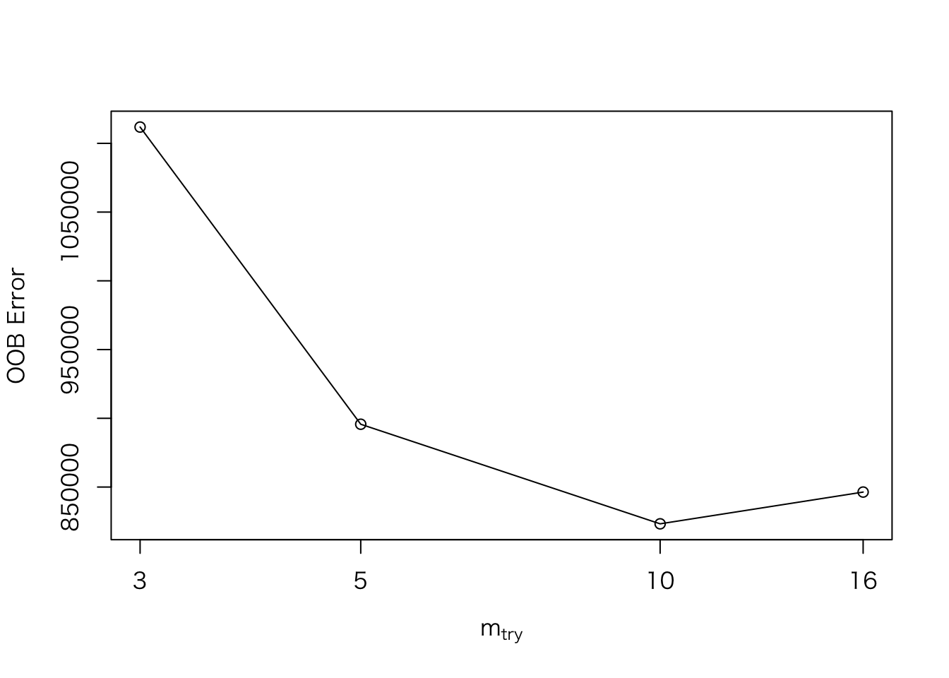

# モデリング
train.rf <- randomForest(Sales ~., data = train, mtry = train.tune$mtry)

モデルの評価（検証用データと予測値の比較）

# 検証用データにモデルを適用
test$pred <- predict(train.rf, test)

# 平均二乗誤差（検証用データのレンンタル数と予測値の離れ具合）でモデル精度を評価
(mean((test$Sales - test$pred) ^ 2)) ^ 1/2

## [1] 501648.4

この数値はいろいろなパターンでモデルを作成し、比較する際に使う。

ggplot(test, aes(x = pred, y = Sales)) +
    geom_point(alpha = 0.6) +
    xlim(0,25000) +
    ylim(0,25000)

## Warning: Removed 29 rows containing missing values (geom_point).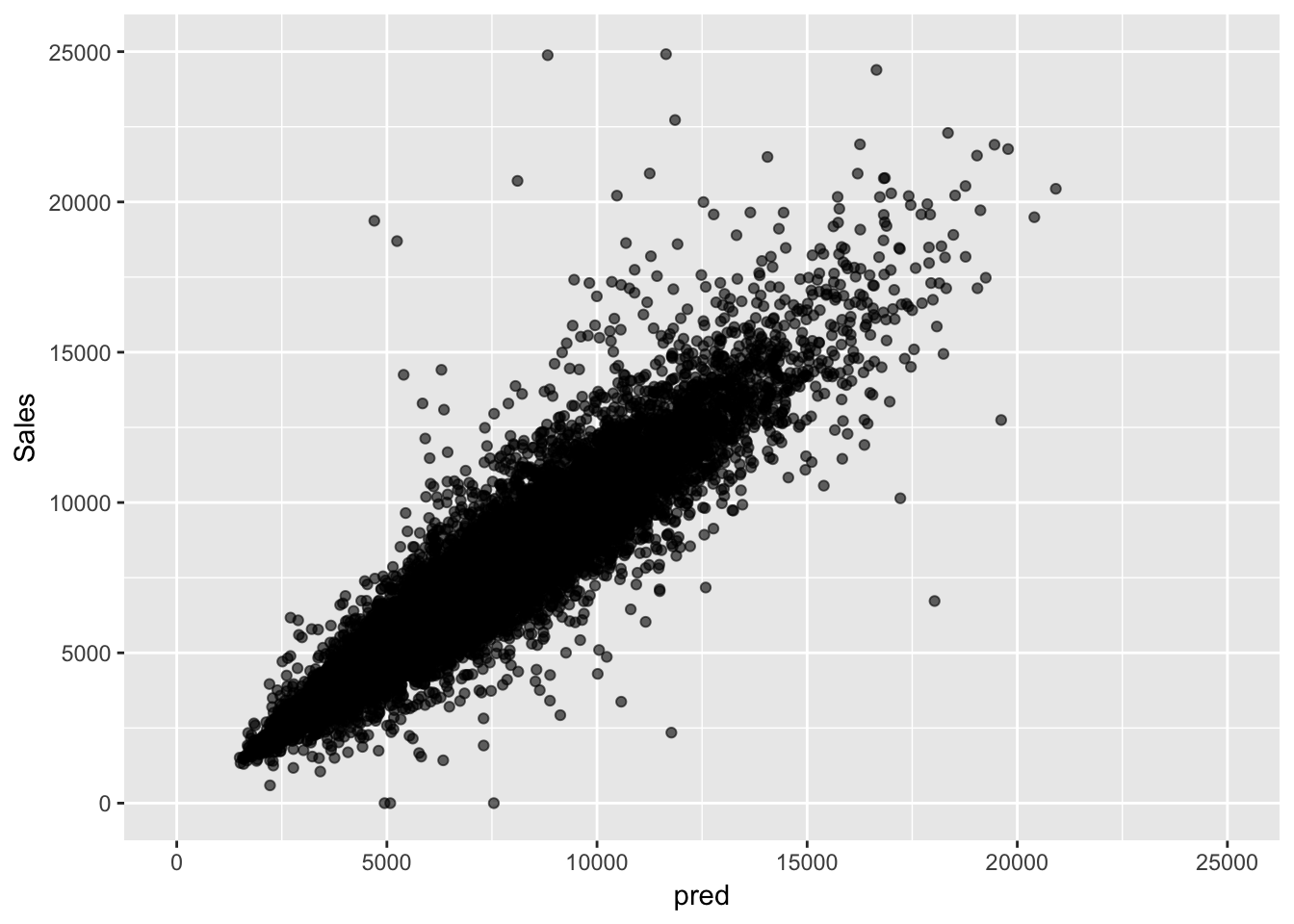

横軸が予測値で、縦軸が検証用データの各店舗の1日あたりの売上です。それなりに予測できているようです。

モデルの内容

各要因の売上への影響度合い

varImpPlot(train.rf)

<< 1.ビジネスの理解　 << 2.データの理解　